Pelican optimization algorithm improved based on hybrid strategy
-
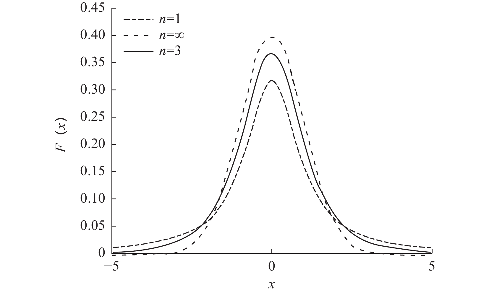
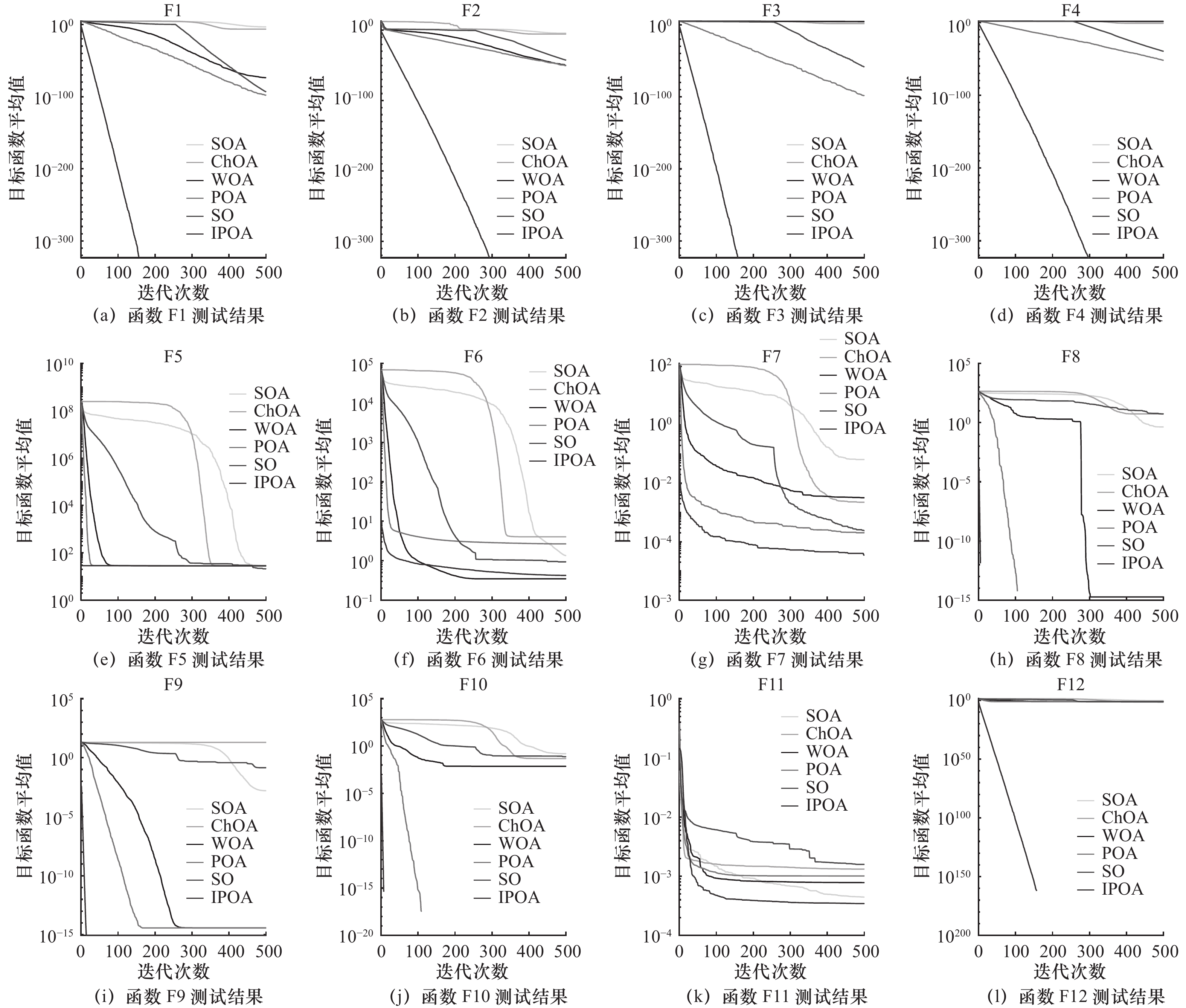
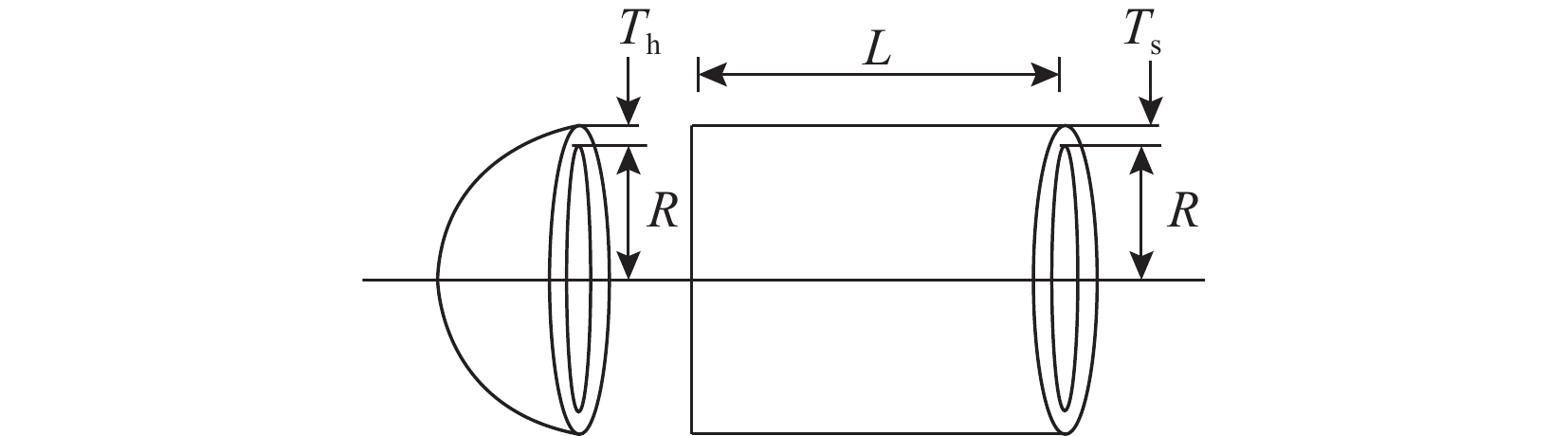
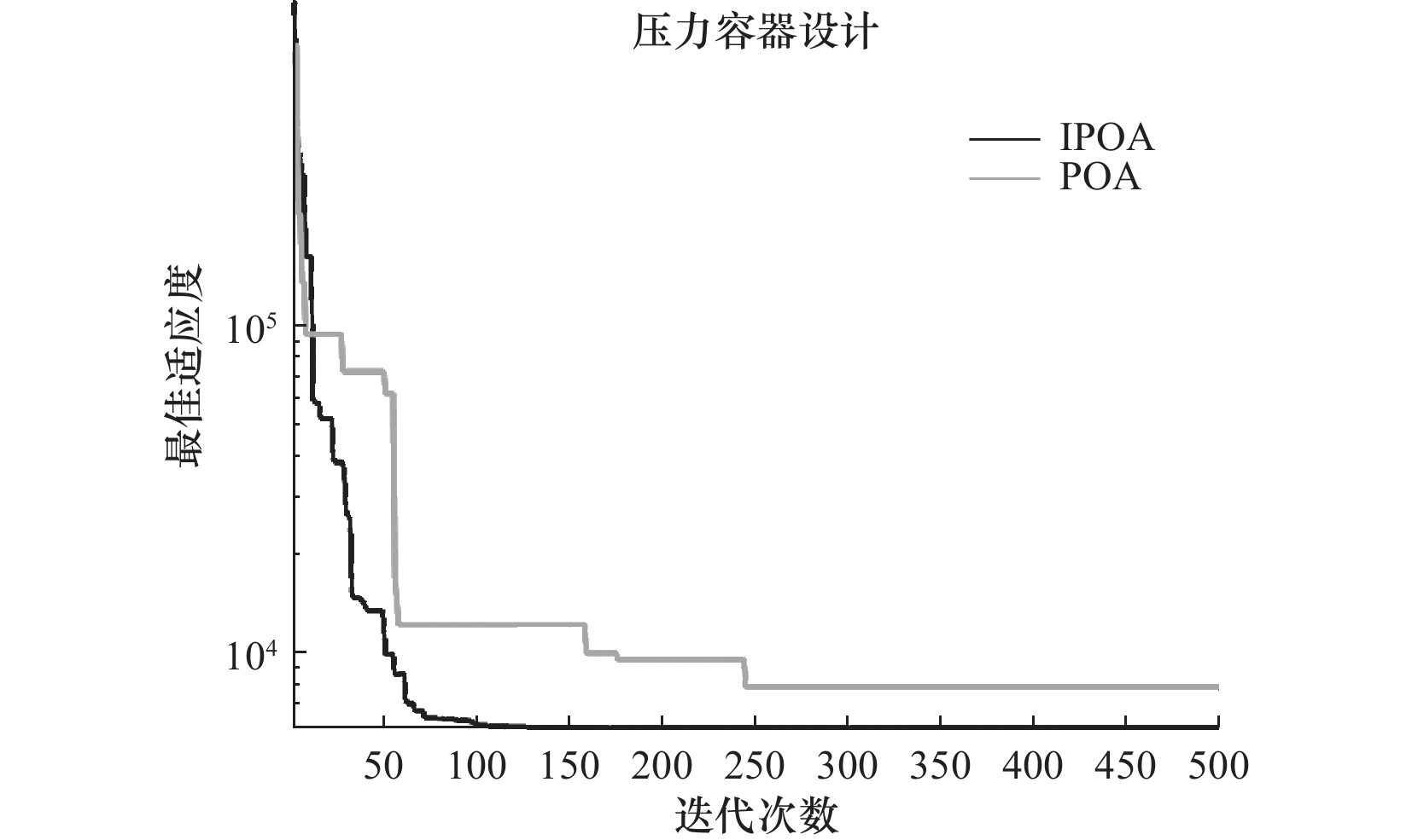
摘要: 针对鹈鹕优化算法求解精度低、稳定性不足、易陷入局部最优等问题,文章提出一种混合策略改进的鹈鹕优化算法(IPOA)。首先,为了增强种群的随机性和多样性,扩大种群的搜索范围,引入反向折射学习机制;其次,利用正余弦算法和鹈鹕算法融合,改进鹈鹕搜索猎物的方式,增强算法的局部搜索与全局搜索能力;然后,采用Levy飞行机制对鹈鹕位置进行更新,从而提高算法的搜索能力以寻找最优值;最后,引入自适应t分布变异算子,使用算法的迭代次数作为t分布的自由度参数来增强鹈鹕种群的多样性,避免算法陷入局部最优。通过12个标准测试函数对改进算法与海鸥优化算法、黑猩猩优化算法、鲸鱼优化算法、蛇群优化算法和基本鹈鹕优化算法进行测试比较,结果表明,IPOA具有更好的收敛速度和稳定性。最后将改进鹈鹕算法应用于压力容器设计优化问题,进一步证实改进后的算法具有较好的求解性能。Abstract: Aiming at the problems of low solving accuracy, insufficient stability, and easy to fall into local optimization of the pelican optimization algorithm, a improved pelican optimization algorithm (IPOA) with improved hybrid strategy is proposed. Firstly, in order to enhance the randomness and diversity of the population, expand the search range of the population, introduce the back-refraction learning mechanism. Secondly, the fusion of sine-cosine algorithm and pelican algorithm is used to improve the way of pelican search for prey, and enhance the local search and global search capabilities of the algorithm. Then, the Levy flight mechanism is used to update the position of the pelican, so as to improve the search ability of the algorithm to find the optimal value. Finally, an adaptive t-distribution variation operator is introduced, and the number of iterations of the algorithm is used as the degree-of-freedom parameter of the t-distribution to enhance the diversity of pelican populations and avoid the algorithm falling into local optimum. The improved algorithm is compared with the seagull optimization algorithm, chimpanzee optimization algorithm, whale optimization algorithm, snake swarm optimization algorithm, and basic pelican optimization algorithm through 12 standard test functions, and the results show that IPOA has better convergence speed and stability. Finally, the improved Pelican algorithm is applied to the pressure vessel design optimization problem, which further proves that the improved algorithm has good solution performance.
-
表 1 12个基准测试函数
函数 表达式 搜索范围 理论最优值 类型 F1 $ f(x) = \displaystyle\sum\limits_{i = 1}^D {x_i^2} \quad $ [−100,100] 0 单峰 F2 $ f(x) = \displaystyle\sum\limits_{i = 1}^D | {x_i}| + \prod\limits_{i = 1}^D | {x_i}| $ [−100,100] 0 单峰 F3 $ f(x) = \displaystyle\sum\limits_{i = 1}^D {{{\left( {\displaystyle\sum\limits_{j = 1}^D {{x_j}} } \right)}^2}} $ [−100,100] 0 单峰 F4 $ f(x) = \max \{ |{x_i}|,1 \leqslant i \leqslant D\} $ [−100,100] 0 单峰 F5 $f(x) = \displaystyle\sum\limits_{i = 1}^D {[100{{({x_{i + 1}} - x_i^2)}^2} + {{({x_i} - 1)}^2}]} $ [−30,30] 0 单峰 F6 $f(x) = \displaystyle\sum\limits_{i = 1}^D {{{([{x_i} + 0.5])}^2}} $ [−100,100] 0 单峰 F7 $f(x) = \displaystyle\sum\limits_{i = 1}^D {ix_i^4 + random[0,1)} $ [−1.28,1.28] 0 多峰 F8 $f(x) = \displaystyle\sum\limits_{i = 1}^D {\left[ {x_i^2 - 10\cos (2{\text{π}} {x_i}) + 10} \right]} $ [−5.12,5.12] 0 多峰 F9 $f(x) = - 20\exp \left( { - 0.2\sqrt {\dfrac{1}{D}\displaystyle\sum\limits_{i = 1}^D {x_i^2} } } \right) - \exp \left( {\dfrac{1}{D}\displaystyle\sum\limits_{i = 1}^D {\cos (2{\text{π}} {x_i})} } \right) + 20 + {\mathrm{e}}$ [−32,32] 0 多峰 F10 $f(x) = \dfrac{1}{{4000}}\displaystyle\sum\limits_{i = 1}^D {{x_i}^2} - \prod\limits_{i = 1}^D {\cos \left( {\dfrac{{{x_i}}}{{\sqrt i }}} \right) + 1} $ [−600,600] 0 多峰 F11 $f(x) = \displaystyle\sum\limits_{i = 1}^{11} {{{\left[ {{a_{ij}} - \dfrac{{{x_1}(b_i^2 + {b_i}{x_2})}}{{b_i^2 + {b_i}{x_3} + {x_4}}}} \right]}^2}} $ [−5,5] 0.003 固定维多峰 F12 $f(x) = 1 - \cos (2{\text{π}} \sqrt {\displaystyle\sum {x^2}} ) + 0.1\sqrt {\displaystyle\sum {x^2}} $ [−100,100] 0 固定维多峰  下载: 导出CSV
表 2 算法的参数设置
算法 参数 ChOA r1=rand(0,1),f=(0,2) SO c1=0.5,c2=0.5,c3=2 WOA b=1,r1=rand(0,1),r2=rand(0,1) SOA fc=2,u=1,v=1 POA I=round(1+rand(1,1)) IPOA I=round(1+rand(1,1))
下载: 导出CSV
表 3 测试函数结果
函数类别 算法类别 最优值 平均值 标准差 F1 SOA 1.2817×10−06 0.00074019 0.0024644 ChOA 7.2276×10⁻¹¹ 5.7943×10−07 1.5957×10−06 WOA 3.1843×10−85 2.134×10−74 7.453×10−74 SO 6.2284×10−99 3.9337×10−94 1.3736×10−93 POA 4.3359×10−116 5.3779×10−99 2.9456×10−98 IPOA 0 0 0 F2 SOA 1.8844×10−06 7.102×10−05 0.00010577 ChOA 1.7949×10−07 5.0017×10−06 7.6574×10−06 WOA 6.1468×10−58 1.1847×10−50 5.0739×10−50 SO 2.2867×10−46 3.1123×10−43 4.5493×10−43 POA 7.4278×10−61 6.8143×10−51 3.2436×10−50 IPOA 0 0 0 F3 SOA 12.722 979.8366 1251.3207 ChOA 0.033222 51.446 95.0067 WOA 18753.5852 43341.6722 15550.335 SO 2.0135×10−66 2.428×10−59 7.055×10−59 POA 3.8683×10−118 2.9871×10−99 1.6082×10−98 IPOA 0 0 0 F4 SOA 0.3055 2.2097 1.8886 ChOA 0.0083578 0.083467 0.08557 WOA 0.019008 49.4673 29.9742 SO 4.6713×10−43 2.3126×10−40 4.0125×10−40 POA 1.584×10−59 1.2775×10−52 3.478×10−52 IPOA 0 0 0 F5 SOA 28.2474 29.5468 2.1301 ChOA 27.3715 28.6896 0.39306 WOA 27.036 28.0725 0.43906 SO 0.20864 20.4655 11.5303 POA 26.3145 27.9957 0.73619 IPOA 27.7267 28.5496 0.1894 F6 SOA 0.64814 1.3556 0.36828 ChOA 3.2598 4.0428 0.37938 WOA 0.046487 0.34955 0.16708 SO 9.2147×10−05 0.93838 0.59081 POA 1.6533 2.6795 0.53552 IPOA 0.24875 0.42499 0.15814 F7 SOA 0.02711 0.065908 0.025239 ChOA 0.0001363 0.0022616 0.0024384 WOA 8.4256×10−05 0.003232 0.0036762 SO 1.1888×10−05 0.00024132 0.00025515 POA 6.1107×10−05 0.00020485 0.00010637 IPOA 8.0705×10−07 3.5086×10−05 3.4089×10−05 F8 SOA 8.0472×10−07 0.46101 1.9764 ChOA 1.5579×10−07 2.7549 4.3314 WOA 0 1.8948×10⁻¹⁵ 1.0378×10⁻¹⁴ SO 0 5.385 12.183 POA 0 0 0 IPOA 0 0 0 F9 SOA 0.00026382 0.0021107 0.0023593 ChOA 19.9609 19.9631 0.00088 WOA 8.8818×10⁻¹⁶ 4.3225×10⁻¹⁵ 2.1847×10⁻¹⁵ SO 4.4409×10⁻¹⁵ 0.22986 0.71194 POA 8.8818×10⁻¹⁶ 4.0856×10⁻¹⁵ 1.084×10⁻¹⁵ IPOA 8.8818×10⁻¹⁶ 8.8818×10⁻¹⁶ 0 F10 SOA 6.4982×10−05 0.1466 0.17616 ChOA 2.2204×10⁻¹⁶ 0.018022 0.030174 WOA 0 0.0046618 0.025534 SO 0 0.079687 0.17691 POA 0 0 0 IPOA 0 0 0 F11 SOA 0.00031889 0.00044598 9.1969×10−05 ChOA 0.0012244 0.0013211 5.857×10−05 WOA 0.00030884 0.00078246 0.0005734 SO 0.00030767 0.0015877 0.0041397 POA 0.00030749 0.0010144 0.0036583 IPOA 0.00030609 0.00034569 6.7507×10−05 F12 SOA 0.2419 0.85384 0.38464 ChOA 0.099873 0.13461 0.045879 WOA 9.098×10−40 0.10657 0.082729 SO 0.099874 0.099962 0.00019438 POA 1.8861×10−49 0.046368 0.048552 IPOA 0 0 0
下载: 导出CSV
表 4 不同改进策略算法的寻优结果对比
函数类别 算法类别 最优值 平均值 标准差 F1 RPOA 1.6971×10−176 1.1547×10−109 5.3196×10−115 SCPOA 1.0343×10−159 0 0 LPOA 0 0 0 TPOA 0 0 0 POA 4.3359×10−116 5.3779×10−99 2.9456×10−98 IPOA 0 0 0 F2 RPOA 1.2451×10−73 3.4845×10−62 1.3756×10−67 SCPOA 1.4055×10−85 2.51×10−62 0 LPOA 0 0 0 TPOA 0 0 0 POA 7.4278×10−61 6.8143×10−51 3.2436×10−50 IPOA 0 0 0 F3 RPOA 2.9033×10−161 5.3846×10−121 2.9487×10−120 SCPOA 0 0 2.3568×10−109 LPOA 0 0 0 TPOA 0 0 0 POA 3.8683×10−118 2.9871×10−99 1.6082×10−98 IPOA 0 0 0 F4 RPOA 6.3066×10−81 1.6851×10−63 5.8057×10−63 SCPOA 0 0 0 LPOA 0 0 0 TPOA 0 0 0 POA 1.584×10−59 1.2775×10−52 3.478×10−52 IPOA 0 0 0 F5 RPOA 26.1742 27.7336 0.69743 SCPOA 27.3715 28.6896 0.39306 LPOA 28.5131 28.8335 0.10808 TPOA 26.1685 27.848 0.667196 POA 26.3145 27.9957 0.73619 IPOA 27.7267 28.5496 0.1894 F6 RPOA 1.3393 2.0406 0.48835 SCPOA 0.24671 2.5789 0.37938 LPOA 1.5833 2.7241 0.53634 TPOA 1.5836 2.6785 0.61492 POA 1.6533 2.6795 0.53552 IPOA 0.24875 0.42499 0.15814 F7 RPOA 5.9051×10−07 2.8631×10−05 2.3605×10−05 SCPOA 0.0001363 0.00022616 0.00024384 LPOA 1.4304×10−07 4.7076×10−05 3.8692×10−05 TPOA 1.4252×10−05 0.0001616 0.00015165 POA 6.1107×10−05 0.00020485 0.00010637 IPOA 8.0705×10−07 3.5086×10−05 3.4089×10−05 F8 RPOA 0 0 0 SCPOA 0 0 0 LPOA 0 0 0 TPOA 0 0 0 POA 0 0 0 IPOA 0 0 0 F9 RPOA 8.8818×10⁻¹⁶ 3.8488×10⁻¹⁵ 0 SCPOA 8.8818×10⁻¹⁶ 8.8818×10⁻¹⁶ 0 LPOA 8.8818×10⁻¹⁶ 8.8818×10⁻¹⁶ 0 TPOA 8.8818×10⁻¹⁶ 8.8818×10⁻¹⁶ 0 POA 8.8818×10⁻¹⁶ 4.0856×10⁻¹⁵ 1.084×10⁻¹⁵ IPOA 8.8818×10⁻¹⁶ 8.8818×10⁻¹⁶ 0 F10 RPOA 0 0 0 SCPOA 0 0 0 LPOA 0 0 0 TPOA 0 0 0 POA 0 0 0 IPOA 0 0 0 F11 RPOA 0.00030749 0.00097991 7.7666×10−09 SCPOA 0.0012244 0.0013211 7.7324×10−05 LPOA 0.00030749 0.00038514 0.00028272 TPOA 0.00030749 0.00037243 0.00023224 POA 0.00030749 0.00037243 0.00023224 IPOA 0.00030609 0.00034569 6.7507×10−05 F12 RPOA 4.6602×10−65 3.2851×10−57 1.1091×10−56 SCPOA 1.5678×10−75 1.1042×10−53 6.0276×10−53 LPOA 0 0 0 TPOA 0 0 0 POA 1.8861×10−49 0.046368 0.048552 IPOA 0 0 0
下载: 导出CSV
表 5 压力容器设计问题求解结果
算法 最优值 平均值 标准差 POA 7456.814 7436.795 935.171 IPOA 5579.147 6553.923 510.168
下载: 导出CSV
-
[1] Trojovsky P,Dehghani M. Pelican optimization algorithm:A novel nature-inspired algorithm forengineering applications[J]. Sensors,2022,22(3):855. doi: 10.3390/s22030855 [2] 董青,陈钰浩,刘永刚,等. 基于优化加点代理模型的桥架结构疲劳寿命预测方法[J]. 机械强度,2023,45(3):729-742. [3] 朱锡山,罗贞,易灿灿,等. 基于POA-CNN-REGST的电梯钢丝绳滑移量预测方法[J]. 机电工程,2023,40(6):928-935. doi: 10.3969/j.issn.1001-4551.2023.06.016 [4] Al-Wesabi F ,Mengash H ,Marzouk R ,et al. Pelican optimization algorithm with federated learning driven attack detection model in internet of things environment[J]. Future Generation Computer Systems, 2023,148:118-127. [5] Song H M,Xing C,Wang J S,et al. Improved pelican optimization algorithm with chaotic interference factor and elementary mathematical function[J]. Soft Computing,2023,27(15):10607-10646. doi: 10.1007/s00500-023-08205-w [6] 高猛,曾宪文. 基于VMD-ESA和IPOA-XGBOOST相结合的异步电机故障诊断[J/OL]. 现代电子技术:1-6[2023-09-19]. http://kns.cnki.net/kcms/detail/61.1224.TN.20230901.1635.002.html. [7] 周建新,郑日成,侯宏瑶. 改进鹈鹕算法优化LSTM的加热炉钢坯温度预测[J]. 国外电子测量技术,2023,42(5):174-179. [8] Tizhoosh H R. Opposition-based learning:a new scheme for machine intelligence [C]. The IEEE International Conference of Intelligent for Modeling, Control and Automation, 2005:695-701. [9] 余修武,黄露平,刘永,等. 融合柯西折射反向学习和变螺旋策略的WSN象群定位算法[J]. 控制与决策,2022,37(12):3183-3189. [10] Mirjalili S. SCA:A since cosine algorithm for solving optimization problems[J]. Knowledge-Based Systems,2016,96:120-133. doi: 10.1016/j.knosys.2015.12.022 [11] 程翠娜,奉松绿,莫礼平. 基于正余弦优化算子和Levy飞行机制的和声搜索算法[J]. 数据采集与处理,2023,38(3):690-703. [12] Viswanathan G M,Afanasyev V,Buldyrev S V,et al. Lévy flights search patterns of biological organisms[J]. Physica A:Statistical Mechanics and its Applications,2001,295(1/2):85-88. [13] 孙珂琪,陈永峰. Lévy飞行的正余弦乌燕鸥混合算法及应用[J]. 机械设计与制造,2023(1):212-217. doi: 10.3969/j.issn.1001-3997.2023.01.046 [14] 王波. 基于自适应 t分布混合变异的人工鱼群算法[J]. 计算机工程与科学,2013,35(4):120-124. doi: 10.3969/j.issn.1007-130X.2013.04.022 [15] 韩斐斐,刘升. 基于自适应 t分布变异的缎蓝园丁鸟优化算法[J]. 微电子学与计算机,2018,35(8):117-121. -

 下载:
下载:


 点击查看大图
图(6) / 表(5)
计量
- 文章访问数: 97
- HTML全文浏览量: 12
- PDF下载量: 28
- 被引次数: 0